Classify

ALOC (short for Allocation) is a highly efficient yet simple classification method from the PATN package (http://www.patn.com.au) designed to classify large volumes of data. Think of ALOC as combining multiple layers of environmental data (e.g. mean annual temperature, slope, and precipitation) into one new layer that captures the essence of all chosen layers.

You select environmental layers and the number of groups required and ALOC produces a map of the resulting groups for the defined area. These groups are called “environmental domains” after work done by Henry Nix (reference below).

Such classifications are done for many reasons. Examples include:

• Understanding the distribution of factors that you have some indication of controlling the distribution of a particular class of organisms. Viewing environmental domains of important factors should provide useful insights.
• Generating a regionalisation for areas where suitable biological data is not available for biodiversity analysis or for reserve design.
• Exploring the relationships between environmental layers.

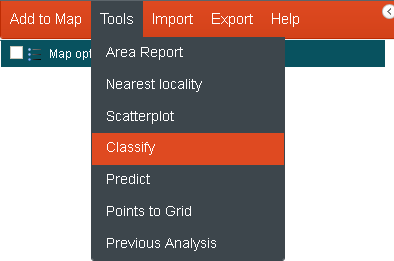
From the menu option, select ‘Tools’, and then ‘Classify’.

Run the Classification Wizard

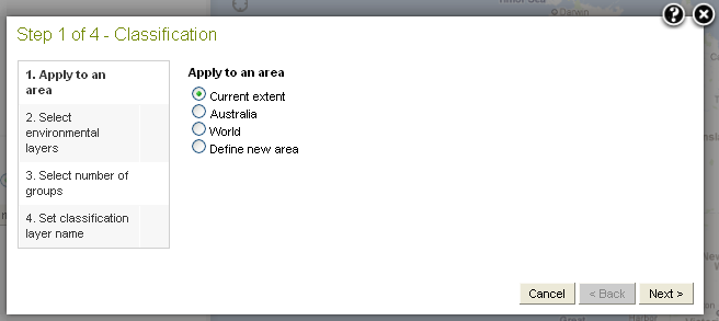
Note the ‘Define new area’ will involve an extra step (please refer to Add Area for additional information).

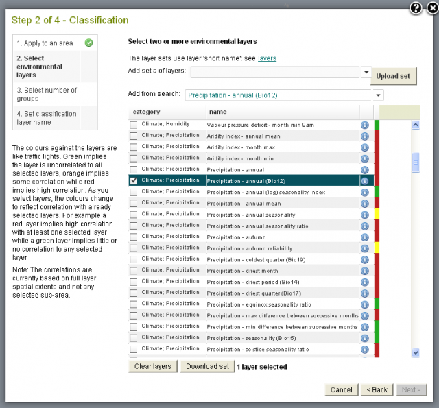
Select two or more environmental layers to be used for the classification. The layers must be environmental (not contextual) and therefore they contain continuous values such as temperature, precipitation or slope. Any number of layers can be selected to be classified. It is however wiser to use fewer layers that you know provide a significant, yet independent signals, but this will depend on the intent of the classification.

The Spatial Portal has over 200 environmental layers covering an extremely wide range of environmental scenarios, that experts believe could have some control on the distribution of organisms. Many of these layers are highly correlated. If highly correlated layers are used, the classification will be weighted accordingly, regardless of how ‘intelligent’ ALOC is.

To assist, the Spatial Portal has built a form of correlation between all environmental layers (see http://spatial.ala.org.au/files/inter_layer_association.csv). It is important to note that the relationship between pairs of layers are calculated on their spatial extent. In most cases, this extent will be the Australian ‘region’ but some layers such as the worldclim (terrestrial) and CARS (marine) layers have near global extent. The comparison between grid cells are made ONLY when both layers have data. This implies that

• Terrestrial layers are not compared with marine layers
• World extent layers will be compared over their full extent
• Australian region extent layers will compared over their Australian extent
• World extent layers will be compared with smaller extent layers over only the smallest spatial extent.

When a layer is added to the classification, the Portal examines the relationship between it and all other environmental layers. It then colour codes the remaining layers in ‘traffic light’ colours. Green against a layer suggests that there appears to be little correlation between that layer and the closest-related selected layer. Orange is intermediate while red suggests that there is a fairly high correlation between the layer and at least one of those already-selected layers. Remember that while there may be a high correlation, a layer may still provide a subtley  different factor that may be important. When a new layer is added, the colours are re-calculated on the basis of the closest relationship to any existing layer added to the classification.

NOTES:

• The layer dissimilarity matrix is updated weekly to reflect new environmental layers.
• The more layers that are selected for Classification, the greater is the likelihood of high correlation between layers producing a biased classification.
• The relationships between the layers has been calculated at the national extents. Layers may therefore be more or less related at different scale
• When the extent of the layers used differs, the extent of the classification layer will be the same as the layer with minimal extent. What this means is that for comparing grid cells, comparisons will only be made when grid cells have a full complement of the selected layers. If you get a surprisingly small extent classification layer – this will be the reason. This effect will most often be seen with marine layers where some have near global coverage while others are limited to the Australian or even just the coastal Australian region.

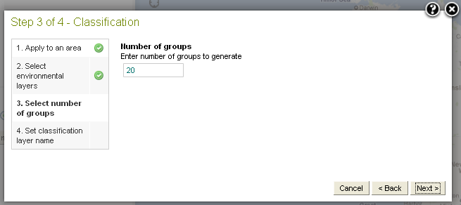
Select the number of groups to be generated in the classification. The greater the number of groups, the finer will be the differences between the environmental domains.

Note: The algorithm may not produce exactly the number of groups requests because that number of groups is unstable. The classification algorithm seeks the closest number of stable groups. If you ask for 20 groups for example, it may produce 21.

Note: The more layers that are used and the larger the Active Area, the longer the analysis will take.

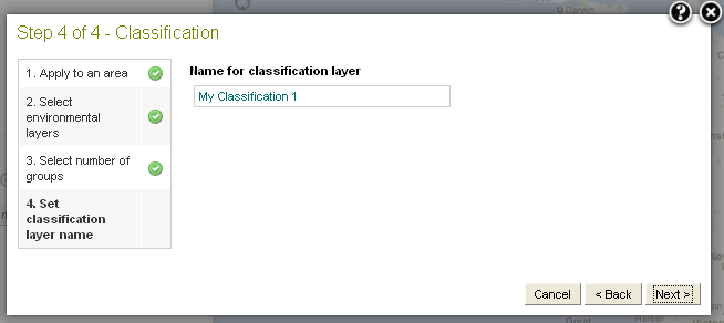
Enter a name for the classification layer.

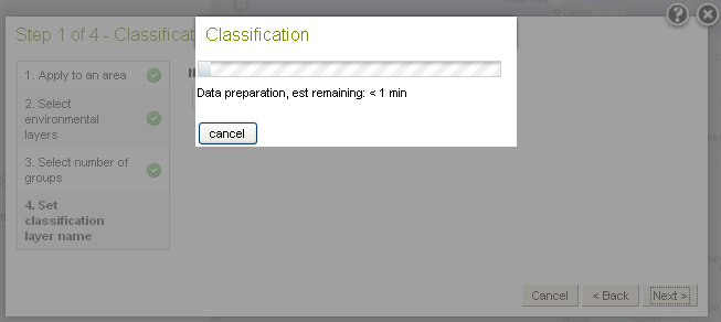
The data preparation progress dialogue box tells you roughly how long it will take before the results are produced.

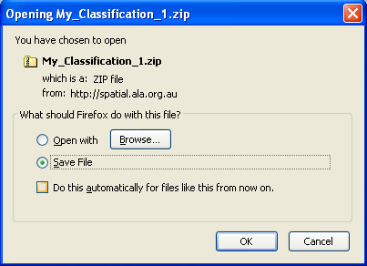
Once completed the Opening My Classification dialogue box will appear. This allows you to open/save your classification.

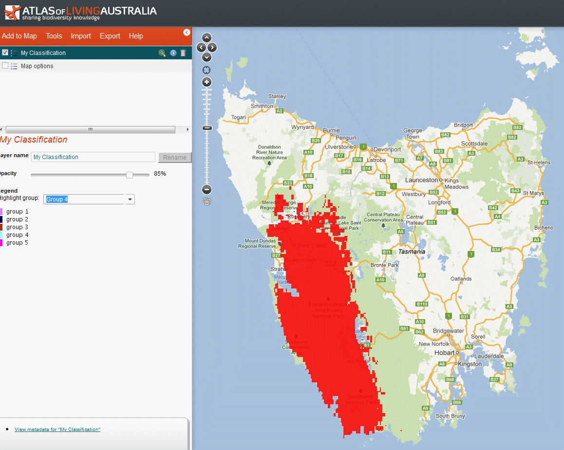
A map will be produced with the requested number of groups. The colours of the groups are not arbitrary: similar group/domain colours indicate similar characteristics; and the reverse is true for very different group colours.

Faceting on Classification groups

When a classification layer is active (its legend is displayed), you can facet on classification groups via its legend. When you want to highlight/identify a single classification group on the map, select that group in the legend and the group will be highlighted in red on the map. The only conrol over the highlight is its transparency. To turn of group fecting, simply select ‘none’ in the facet drop down in the legend.

 

Metadata

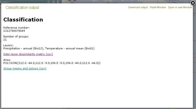
When the layer metadata icon icon is clicked in the layers list the metadata popup is displayed for the Classification layer. The metadata can be displayed in a separate window.

• Each model is assigned a unique identifier that allows it to be displayed in subsequent sessions e.g. Reference number: 1312786878649. This value is given in the metadata of the layer. The Restore Prior Analysis tool uses this identifier to restore a model created earlier. It can be from a totally different session, browser or even PC.
• The number of final groups. This can be slightly different from the number of groups requested. This occurs if the classification does not naturally fit the selected number of groups.
• The layers used in the Classification.
• The ‘inter-layer dissimilarity matrix’. This matrix shows the ‘environmental distance’ between all pairs of layers. Values close to zero mean that they layers are closely related (a small distance apart in environmental space) while values near one mean that the layers have no relationship – they are independent.
• Active Area polygon – the bounding box’s longitudes and latitudes. The definition at the time of the classification is listed.
• Group means and colours. This is a CSV (comma-separated values) formatted file with one record for each group and with the following columns:
  • Group number
  • Red, green and blue saturation. The colours relate to the characteristics of the groups.
  • Layer values. Each Layer used in the classification will be represented by a mean for each group. This is the ‘stereotype’ of the group.

Steps used by ALOC to produce a Classification

1. Build a set of seed groups that are greater than a threshold distance apart (using Gower Metric).
2. Allocate all points on the map to the seed groups.
3. Calculate the group centroids.
4. Iterate by removing each point from its allocated group, calculate the association (Gower metric) to all groups and then allocate it to the closest group.
5. Repeat 4 until no points change groups.
6. The colours are produced by a Principal Component Analysis using the inter-group distances (dissimilarity based on all the layers).

NOTE: When environmental layers selected for the classification do not have the same spatial extent, the classification will only be performed on grid cells that contain values for all layers. If this occurs, the resulting classification layer will only cover the area of the layer with the smallest spatial extent (area). While comparisons between grid cells could be made taking available data into account, it was deemed expedient to remove such cells as in many GIS circumstances, the classification could be  extremely biased if such cells were included.

A case study

A case study on using the Classification Tools to investigate the classification of landscapes in Australia, is given by Prof Brendan Mackey of the Australian National University, Canberra.

Read the Case Study »

Referenced Links

Belbin, Lee, Marshall, C. and Faith, D.P. (1983). Representing relationships by the automatic assignment of colour. Australian Computer Journal, vol. 15, no. 4, pp. 160-163.

Belbin, L. (1987). The Use of Non-hierarchical Allocation Methods for Clustering Large Sets of Data. Australian Computing Journal, vol. 19, no. 1, pp. 32-41.

Gower J.C. (1967). Multivariate analysis and multidimensional geometry. The Statistician, vol. 17, no. 1, pp. 13-28.

Nix, H.A. (1986). A biogeographic analysis of Australian elapid snakes, In: Atlas of Elapid Snakes of Australia. (Ed.) R Longmore, pp. 4-15. Australian Flora and Fauna Series Number 7. Australian Government Publishing Service: Canberra.