Generalised Dissimilarity Modelling (GDM)
This is one of the most complex tools within the Spatial Portal. Inputs to this tool are usually a species assemblage (at a higher taxonomic level) and a suite of environmental layers. The primary outputs from GDM are the input environmental layers transformed to best-align with the spatial distribution of records from the species assemblage. See References for details on the algorithm used.
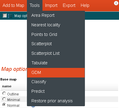
From the menu option, select ‘Tools’, and then ‘GDM’.
Run the GDM wizard

Note the ‘Define new area’ will involve an extra step (please refer to Add Area for additional information). In this example the state of Victoria has been pre-defined and selected from the ‘States including coastal waters’ contextual layer.
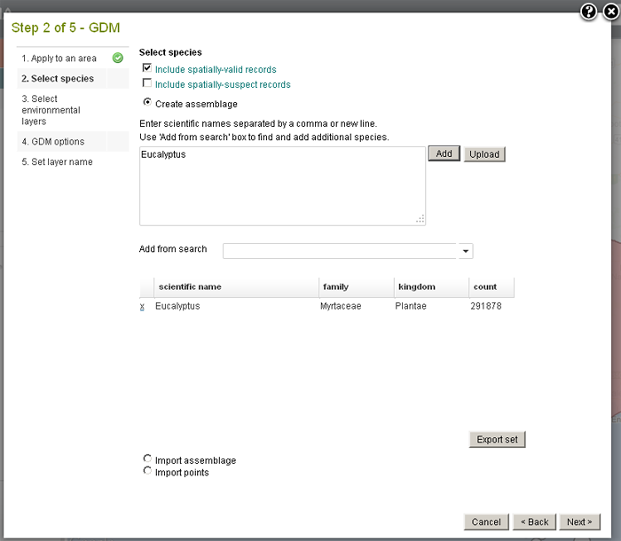
The modelling will use species density, so the more comprehensive and consistent the occurrence records are, the better the results will be. It is best to select taxa at the genus or higher taxonomic level to get better coverage.
Note: For GDM to run, there must be multiple occurrences of the same taxa. If the input data contains only one record of any taxon, an error message will be generated.
Species assemblages and the import of species location points are also means for creating the necessary points on the map for analysis.
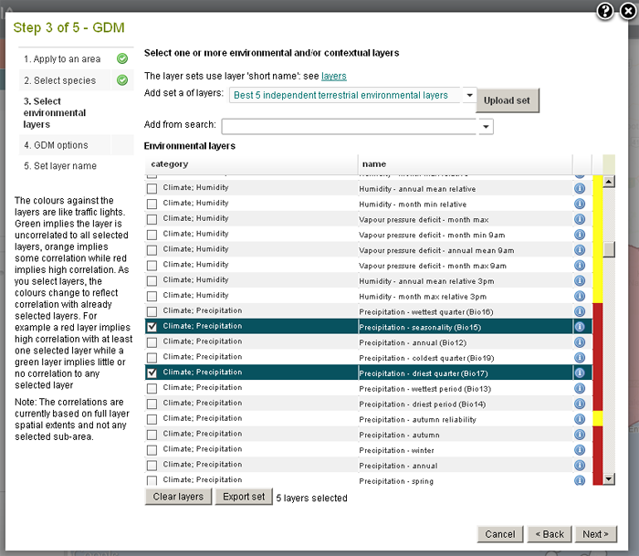
There are many ways to select the environmental layers. You can take a quick look using the best five independent terrestrial layers (for GDM modelling the more distinct the better). You can also use any previous layer selections, search for layers, past in a set of layer names or select them individually in the list of environmental layers. If you search for layers remember that you can also search on layer keywords, for example ‘marine’ or ‘2030’.
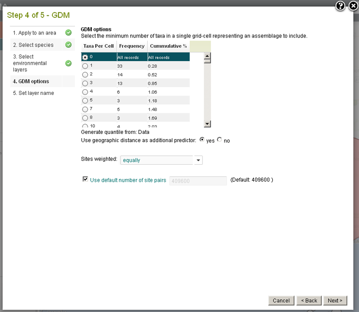
Cells can be filtered by selecting the minimum number of taxa per cell that will be included in GDM.
GDM can be run using equal weighting of cells or a weighting based on the number of taxa per site.
The time taken for GDM to run can be considerable so consider sending it to a background task. To reduce the run time, select a smaller percentage of the site-wise pairs to be used.
The spatial distance between species can also be accounted for in the modelling by choosing to use geographic distance as a predictor.
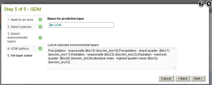
The zipped file of results are produced.

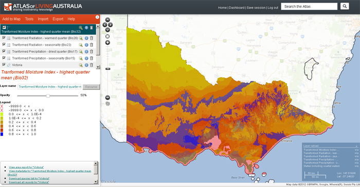
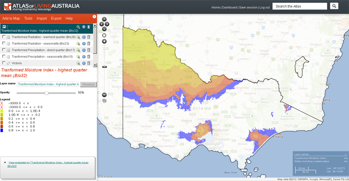
The above image shows all the chosen transformed layers overlaid upon each other. Obviously, each layer should be viewed independently.
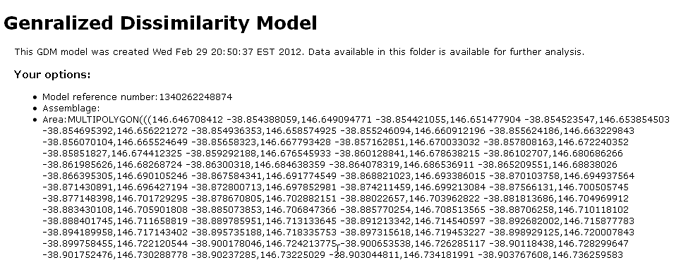
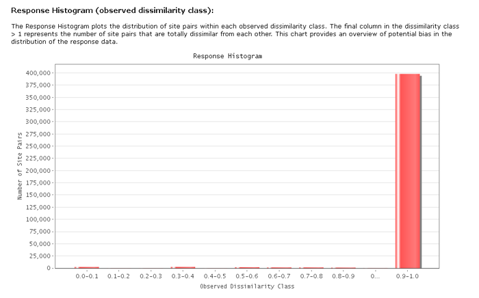
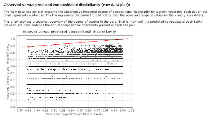
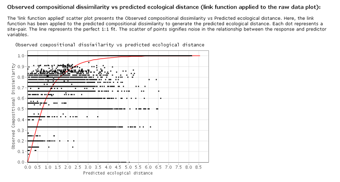
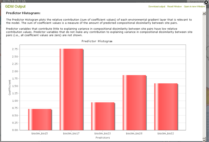
When the layer metadata icon ![]() icon is clicked in the layers list (on the top left) the output from GDM will be displayed showing various statistics such as the contribution of each input layer. This information can be displayed in a separate window.
icon is clicked in the layers list (on the top left) the output from GDM will be displayed showing various statistics such as the contribution of each input layer. This information can be displayed in a separate window.
Explanation of the Fitted Functions
The model output presents the response (compositional turnover) predicted by variation in each predictor. The shape of the predictor is represented by three I-splines, the values of which are defined by the environmental data distribution: min, max and median (i.e., 0, 50 and 100th percentiles). The GDM model estimates the coefficients of the I-splines for each predictor. The coefficient provides an indication of the total amount of compositional turnover correlated with each value at the 0, 50 and 100th percentiles. The sum of these coefficient values is an indicator of the relative importance of each predictor to compositional turnover.
The coefficients are applied to the ecological distance from the minimum percentile for a predictor. These plots of fitted functions show the sort of monotonic transformations that will take place to a predictor to render it in GDM space. The relative maximum y values (sum of coefficient values) indicate the amount of influence that each predictor makes to the total GDM prediction.
Functions and variables used to transform the layers
Example Layers for Victorian Eucalyptus:
- Precipitation – driest quarter (Bio17)
- Precipitation – seasonality (Bio15)
- Radiation – seasonality (Bio23)
- Radiation – warmest quarter (Bio26)
- Moisture Index – highest quarter mean (Bio32)
References
Ferrier, S. and Guisan, A. (2006). Spatial modelling of biodiversity at the community level. Journal of Applied Ecology 43, 393-404.
Ferrier, S., Manion, G., Elith, J. and Richardson, K. (2007). Using generalized dissimilarity modelling to analyse and predict patterns of beta diversity in regional biodiversity assessment. Diversity and Distributions, 13, 252-264.